论文题目: SSD: Single Shot MultiBox Detector
论文作者: Wei Liu, Dragomir Anguelov, Dumitru Erhan, Christian Szegedy, Scott Reed, Cheng-Yang Fu, Alexander C. Berg
提交时间: 2015.12.8(v1), 2016.12.29 (this version, v5)
本文回答以下几个问题
-
SSD的网络结构是怎么样的? 特征提取基础网络 + 检测器
-
SSD的关键之处(特别之处)是什么?
-
检测器是如何实现的, 即如何实现定位与分类?
检测器是卷积层, 即基于conv4_3, fc_7, conv6_2, conv7_2, conv8_2, conv9_2的特征, 使用核为3×3的卷积层分别预测bbox offset(关于default box)与cls prob
-
SSD中的default boxes
-
default boxes与Faster R-CNN中的anchor box是一样, 不同是:
-
anchor boxes: 基于一个conv feature map, 通过生成不同scale与aspect ratio的anchor boxes, 实现多尺度的预测
-
default boxes: 基于多个不同size的conv feature maps, 通过生成多个不同aspect ratio的default boxes, 实现多尺度的预测
-
-
aspect ratio的选择
-
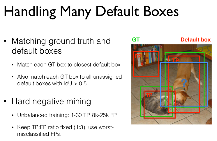
如何处理大量的default boxes? 如何为default boxes匹配gt boxes
-
-
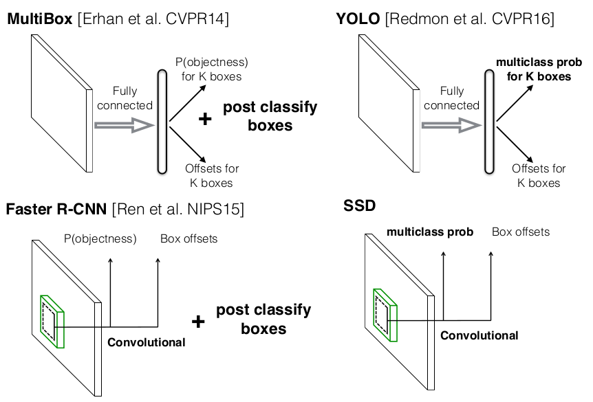
SSD与Faster R-CNN, YOLO相比, 有何不同
-
SSD的Loss函数是怎么样的?
-
SSD的训练技巧
SSD architecture
SSD(deploy time)的整体架构为特征提取基础网络 + 检测器, 结构如下图所示
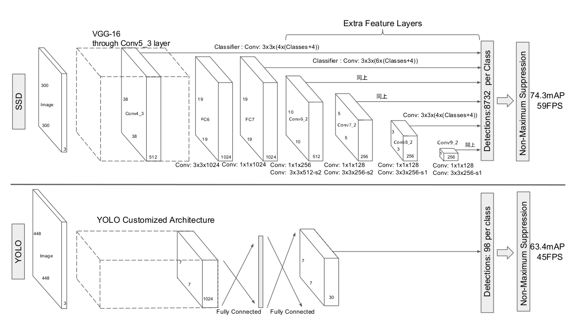
需要说明, 上图来自SSD论文配图, 为与源码保持一致, 做了修改, 把
conv6(FC6)改为FC6, 把conv7(FC7)改为FC7, 把conv8_2改为conv6_2, 把conv9_2改为conv7_2, 把conv10_2改为conv8_2, 把conv11_2改为conv9_2
SSD作为目标检测模型, 其特别之处是基于多个不同size的feature map, 利用卷积层直接进行预测
特征提取基础网络
特征提取基础网络为VGG-16, 并做了改动, 具体为
- 对VGG-16做了修改
- 修改conv5_3之后的pool5:
maxpool 2×2-p0-s2 --> maxpool 3×3-p1-s1, 这使得feature size保持不变 - 修改FC6(-4096)为卷积层:
fully-connected layer --> convolution layer 3×3-p6-s1-f1024-dilation6, 使用了 dilated convolution, 这样的设置使得feature size保持不变,关于dilated convolution, 请看附录1疑问: 为何要设置上述convolution layer, 设置成
3×3-p1-s1-f1024, 不也可以保证feature size不变吗? - 修改FC7(-4096)为卷积层:
fully-connected layer --> convolution layer 1×1-p0-s1-f1024 - 删去FC-1000, Softmax layer
下面保持修改后的pool5, FC6, FC7的记号, 与原来一致.
- 修改conv5_3之后的pool5:
-
在以上修改的基础上, 在FC7之后增加了8个卷积层, 具体如下:
Layer Input Kernel size padding strides #kernels Output conv6_1 N×1024×19×19 1×1 0 1 256 N×256×19×19 conv6_2 N×256×19×19 3×3 1 2 512 N×512×10×10 conv7_1 N×512×10×10 1×1 0 1 128 N×128×10×10 conv7_2 N×128×10×10 3×3 1 2 256 N×256×5×5 conv8_1 N×256×5×5 1×1 0 1 128 N×128×5×5 conv8_2 N×128×5×5 3×3 0 1 256 N×256×3×3 conv9_1 N×256×3×3 1×1 0 1 128 N×128×3×3 conv9_2 N×128×3×3 3×3 0 1 256 N×256×1×1
检测器
基于多个不同size的feature map, 生成default boxes(记为PriorBox), 利用核为3×3的卷积层进行预测关于default box的bbox offset(记为loc), confidence scores(记为conf)
具体流程为
- 基于conv4_3, fc7, conv6_2, conv7_2, conv8_2, conv9_2的feature map, 生成default boxes(记为PriorBox), 同时构建6个检测器
在每个location生成
k个default boxes - 每个检测器分别预测关于default box的bbox offset(记为loc), confidence scores(记为conf)
对于每个location上的每个default box, 预测
4个bbox offsets(关于default box, 含x,y,w,h的offset)及C个class probs, 其中C表示预测的object类别, 如VOC是C=21 - 之后分别把上述各个检测器预测的loc, conf串联起来, 同时也把PriorBox串联起来
- 根据loc及其对应的PriorBox, 得到predicted bboxes, 同时每一个predicted bbox都带有conf
- 根据conf, 对上述predicted bboxes进行排序, 并做NMS, 过滤大部分的predicted bboxes, 得到最终的检测结果
下面以基于conv4_3的检测流程为例进行详述, 具体看下图

需要说明的是, 基于fc7, conv6_2, conv7_2, conv8_2, conv9_2的检测中没有
Normalize操作, 其他的与基于conv4_3的检测流程一样

default box
| 卷积层 | aspect_ratio | flip | 在每个location生成的default boxes个数 |
|---|---|---|---|
| conv4_3 | 2 | True | 4 |
| fc_7 | 2, 3 | True | 6 |
| conv6_2 | 2, 3 | True | 6 |
| conv7_2 | 2, 3 | True | 6 |
| conv8_2 | 2 | True | 4 |
| conv9_2 | 2 | True | 4 |
注1: flip=True表示将aspect ratio的倒数记入aspect ratio
注2: aspect_ratio默认含有1
注3: 当aspect_ratio=2, flip=True时, 此时在每个location生成的default boxes有4个, 其中属于aspect_ratio=1的有2个, 属于aspect_ratio=2的有1个,属于aspect_ratio=1/2的有1个. 具体可看下面default box的生成过程
default box的生成
遍历conv feature map的所有location, 依据所给参数, 在每一个location上生成若干个default boxes
下面以在location(h,w)上生成default boxes为例,源码见github上SSD源码prior_box_layer.cpp
- 计算boxes中心点坐标: 根据
h, w, offset, step, 计算中心点坐标. (注: 在该location生成的boxes中心都是同一个)
  float center_x = (w + offset_) * step_w;
  float center_y = (h + offset_) * step_h;
- 求box的左上顶点, 右下顶点坐标: 根据mini_size, max_size, aspect_ratio, 得到box_width, box_height,进而计算得到两个顶点坐标,
计算公式为
  xmin = (center_x - box_width / 2.) / img_width;
  ymin = (center_y - box_height / 2.) / img_height;
  xmax = (center_x + box_width / 2.) / img_width;
  ymax = (center_y + box_height / 2.) / img_height;
其中box_width, box_height有三类:
- first prior:
aspect_ratio = 1, size = min_size, 此时box_width = box_height = min_size; - second prior:
aspect_ratio = 1, size = sqrt(min_size * max_size),此时box_width = box_height = sqrt(min_size_ * max_size_); - third prior:
其他aspect_ratio, ar_1, ..., ar_k, 此时box_width = min_size_ * sqrt(ar); box_height = min_size_ / sqrt(ar); - 如果
clip=True,则使上述所有default boxes的坐标xmin,ymin,xmax,ymax都属于[0, 1], 即xmin = min(max(xmin, 0.), 1.); # 其他类似 - 为所有default boxes的坐标添加对应的variance, 坐标的variance在另一个channel上.
需要注意的是, 生成priorbox过程中使用了很多的参数, 这些参数都是人工设置的.
训练时, 如何处理default boxes
training objective function
个人认为论文里的目标函数写得不够严谨, 待看源码
SSD与MultiBox, Faster R-CNN, YOLO的对比
附录1–关于convolutional parameters——dilation参数的说明
caffe.proto中ConvolutionParameter有一个参数dilation
// Factor used to dilate the kernel, (implicitly) zero-filling the resulting
// holes. (Kernel dilation is sometimes referred to by its use in the
// algorithme à trous from Holschneider et al. 1987.)
repeated uint32 dilation = 18; // The dilation; defaults to 1
另外, 在caffe源码conv_layer.cpp中可以看到dilation参数的作用
void ConvolutionLayer<Dtype>::compute_output_shape() {
  const int* kernel_shape_data = this->kernel_shape_.cpu_data();
  const int* stride_data = this->stride_.cpu_data();
  const int* pad_data = this->pad_.cpu_data();
  const int* dilation_data = this->dilation_.cpu_data();
  this->output_shape_.clear();
  for (int i = 0; i < this->num_spatial_axes_; ++i) {
    // i + 1 to skip channel axis
    const int input_dim = this->input_shape(i + 1);
    const int kernel_extent = dilation_data[i] * (kernel_shape_data[i] - 1) + 1;
    const int output_dim = (input_dim + 2 * pad_data[i] - kernel_extent)
        / stride_data[i] + 1;
    this->output_shape_.push_back(output_dim);
  }
}
dilated convolution, also known as Atrous convolution,
简单地来说, 在原有filter kernel的值之间插入 dilation -1 个 0, 使kernel扩张, 它保证了参数的不增加,
又提供了灵活的机制来控制感受野(来自论文DeepLab)
当dilation=1时, 为standard convolution
It thus offers
an efficient mechanism to control the field-of-view and
finds the best trade-off between accurate localization (small
field-of-view) and context assimilation (large field-of-view)
即将kernel进行扩张, 具体如下图所示(来源)
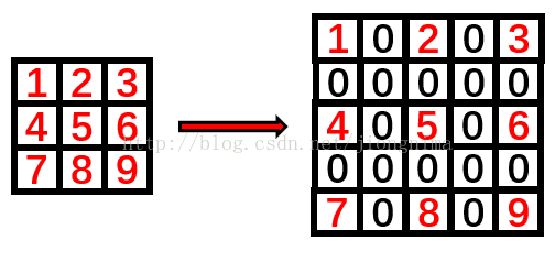
扩张后核大小的计算公式为
附录2–Permute layer的说明
Permute layer is used to make it easier to combine predictions from different layers by changing from
N x C x H x W to N x H x W x C
so that the first C elements are predictions at position (0, 0), and the second C elements are for (0, 1) etc.
What’s more, because predictions from different layer are of different spatial resolution,
I use flatten to make it N x HWC x 1 x 1 so that it is easy to combine.
These are some implementation (engineering) details, which are ignored in the paper.
来自github上作者的回答
这是作者在工程实现上的一个小技巧。 因为SSD最终要把6个层的预测输出整合起来,这样在数据shape上面需要一致,这一点用flatten就可以做到。 permute这一步的设计就是为了让数据的结构更elegant。通过permute之后shape为NxHxWxC,再经过flatten之后shape为NxHWCx1x1, 这样的形状表示每C个数据表示在当前feature map上一个点的信息,这样设计就比较清晰。 回答来源
附录3–关于prior_box_layer中的prior_box_param参数说明
layer {
  name: "fc7_mbox_priorbox"
  type: "PriorBox"
  bottom: "fc7"
  bottom: "data"
  top: "fc7_mbox_priorbox"
  prior_box_param {
    min_size: 60.0
    max_size: 111.0  # 仅用于生成aspect_ratio=1的一种default box
    # 这里有两个aspect_ratio, 为`2,3`
    aspect_ratio: 2.0
    aspect_ratio: 3.0
    flip: true  # `flip=True`表示将`aspect_ratio的倒数`记入`aspect_ratio`
    clip: false # if true, clip the prior's coordidate such that it is within [0, 1]
    variance: 0.10000000149  # 属于xmin的variance
    variance: 0.10000000149  # 属于ymin的variance
    variance: 0.20000000298  # 属于xmax的variance
    variance: 0.20000000298  # 属于ymax的variance
    step: 16.0  # 用于计算default box的中心, 表示中心移动的step
    offset: 0.5  # 用于计算default box的中心, 表示中心的偏移量
  }
}
https://zhuanlan.zhihu.com/p/40968874
