目标检测文献阅读与理解之YOLOv1

论文题目: You Only Look Once: Unified, Real-Time Object Detection

论文作者: Joseph Redmon, Santosh Divvala, Ross Girshick, Ali Farhadi

提交时间: 2015-06-08(v1), 2016-05-09(v5, 最后修改版))

detection

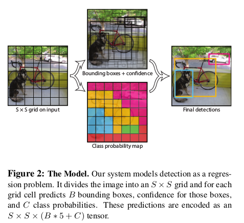
yolo detection流程图如下:

1. each image被分成 S × S grid cells

2. each cell预测 B 个 predicted bbox（即 (x, y, w, h, confidence) ) , C 个 conditional class probabilities

• 注1. 把each image 分成 S × S grid cells, 是指 each image 通过 CNNs 与 FCs 之后 会得到 一个 S × S × （B × 5 + C） 张量, 即 each grid cell 都有 B 个 predicted bbox（即 (x, y, w, h, confidence) ) , C 个 conditional class probabilities.

• 注2. predicted bbox 的 confidence 被定义为

$$\text{confidence} \triangleq \text{Pr(object)} * \text{IoU}_\text{pred}^\text{truth},$$

其中

$$\text{Pr(object)}=\bigg\{\begin{aligned} 1&,\quad \text{ if the center of object is in this cell;}\\ 0&, \quad \text{othervise}. \end{aligned}$$

and, $\text{IoU}_\text{pred}^\text{truth}$ represents the intersection over union between the predicted box and the ground box(object).

Based on the definition of confidence, this confidence reflects:

1. $\text{Pr(object)}$: how confident the model is that this predicted box contains an object.

2. $\text{IoU}_\text{pred}^\text{truth}$: how accurate the model thinks that the predicted box is that it predicts.

• 注3. Conditional class probability, $ \text{Pr} \left( \text{Class}_i \vert \text{Object} \right) $. These probabilities are conditioned on the grid cell containing an object. Only predict one set of class probabilities per grid cell, regardless of the number of boxes B.

• 注4. At the test time, multipy the conditional class probabilities and the individual box confidence predictions,

$$\text{Pr} \left(\text{Class}_i \vert \text{Object} \right) * \text{Pr(object)} * \text{IoU}_\text{pred}^\text{truth} = \text{Pr} \left(\text{Class}_i \right) * \text{IoU}_\text{pred}^\text{truth},$$

which gives class-specific confidence scores for each box. These scores encode the probability of that class appearing in the box and how well the predicted box fits the object.

$Loss$ 函数

依据原文 $Loss$ 函数, 基于我的理解, 将 $Loss$ 函数写为如下, 需要提醒的是, 虽然下面 $Loss$ 中每一项都是两重连加, 关于cell, 关于cell的boxes, 但是实质上是一重, 因为连加号里都有示性函数.

$$\begin{aligned} Loss =& \quad \lambda_\text{coord} \sum_{i=1}^{S^2} \sum_{j=1}^{B} \mathbb{1}_{ij}^\text{obj}\left[(x_i - \hat{x}_{ij})^2 + (y_i - \hat{y}_{ij})^2 \right] \quad --(x\text{-}y \textit{ section}) \\ & + \lambda_\text{coord} \sum_{i=1}^{S^2} \sum_{j=1}^{B} \mathbb{1}_{ij}^\text{obj} \left[ \left({w_i}^{1/2} - {\hat{w}_{ij}}^{1/2} \right)^2 + \left({h_i}^{1/2} - {\hat{h}_{ij}}^{1/2} \right)^2 \right] \quad --(w\text{-}h \textit{ section})\\ & + \sum_{i=1}^{S^2} \sum_{j=1}^{B} \mathbb{1}_{ij}^\text{obj}\left(C_i - \hat{C}_{ij} \right)^2 \quad (\text{actually, } C_i = 1 ) \quad --(\textit{obj confidence section}) \\ & + \lambda_\text{noobj} \sum_{i=1}^{S^2} \sum_{j=1}^{B} \mathbb{1}_{ij}^\text{noobj}\left(C_i - \hat{C}_{ij} \right)^2 \quad (\text{actually, } C_i = 0 ) \quad --(\textit{noobj confidence section})\\ & + \sum_{i=1}^{S^2} \mathbb{1}_{i}^\text{obj} \sum_{i\in \text{classes} } \left( p_i(c) - \hat{p_{i}}(c) \right)^2 \quad --(\textit{class probs section}) \end{aligned}$$

其中,

$$\mathbb{1}_{i}^\text{obj} = \bigg\{\begin{aligned} 1&,\quad \text{if the center of a gt box is in cell} \, i \text{;}\\ 0&, \quad \text{othervise}. \end{aligned}$$ $$\mathbb{1}_{ij}^\text{obj} = \bigg\{\begin{aligned} 1&,\quad \text{if box}\, j \,\text{in cell}\, i \,\text{is responsible for a gt box;}\\ 0&, \quad \text{othervise}. \end{aligned}$$ $$\mathbb{1}_{ij}^\text{noobj} = \bigg\{\begin{aligned} 1&,\quad \text{if }\, \mathbb{1}_{ij}^\text{obj} = 0;\\ 0&, \quad \text{if }\, \mathbb{1}_{ij}^\text{obj} = 1. \end{aligned}$$

当某个 gt box 的中心位于 cell $i$内, 在此前提下, 在该 cell 的所有 box 中, box $j$ 与 该 gt box 的 IoU 是最大的,

较原文, 上述$Loss$有两类改动或添加:

把 $i=0, j=0$ 全部分别改为 $i=1, j=1$, 我认为这样更符合数学表达, 虽然c语言中索引起始是0

添加下标 $j$： 将$\hat{x}_i, \hat{y}_i, \hat{w}_i, \hat{h}_i, \hat{C}_i$ 全部分别改为$\hat{x}_{ij}, \hat{y}_{ij}, \hat{w}_{ij}, \hat{h}_{ij}, \hat{C}_{ij}$ , 因为在我看来, 这样更符合表达, 利于理解. 需要注意的是, 用一个下标$i$, 也没有原则问题, 因为training时每个grid cell 中至多只有一个predicted box会进入到$Loss$函数中的(x,y)、(w,h)、obj confidence 三个section.

$Loss$ 函数的几处考虑

1. set $\lambda_\text{coord}=5, \, \lambda_\text{noobj}=0.5$, 这有两点原因:

   • do not weight localization error equally with classification error.

   • in every image many grid cells do not contain any object. This pushes the “confidence” scores of those cells towards zero, often overpowering the gradient from cells that do contain objects. This can lead to model instability, causing training to diverge (发散) early on.

   To remedy the above two points, we increase the loss from bounding box coordinate predictions and decrease the loss from confidence predictions for boxes that don’t contain objects. We use two parameters, $\lambda_\text{coord}$ and $\lambda_\text{noobj}$to accomplish this.

   定位误差的系数 $\lambda_\text{coord}(=5)$大于其他误差项系数(为$1或0.5$) , 即增大了定位误差在 $Loss$ 中的权重

   不对预测负责的confidence误差项系数$\lambda_\text{noobj}$(为$0.5$), 小于其他误差项系数(为$1或5$), 即降低了不对预测负责的confidence误差项在$Loss$中的权重

2. 采用 $w^{1/2},h^{1/2}$, 而不是一次项

   这是考虑到Our error metric should reflect that small deviations in large boxes matter less than in small boxes. To partially address this we predict the square root of the bounding box width and height instead of the width and height directly

   在靠近原点的地方, 1/2次幂函数的梯度变化显然比一次项函数的更大. 从而, 1/2次幂函数较一次函数可以更好地反映：小变化对小目标的影响更显著.

$Loss$ 函数计算流程图

下面针对each grid cell（下面简称为“cell”）整理$Loss$函数计算流程.

注1. 当 all of gt boxes’ center is not in the cell $i$ 时, $\mathbb{1}_i^\text{obj} = 0, \quad \mathbb{1}_{ij}^\text{obj}=0 (j = 1, ... ,B), \quad \mathbb{1}_{ij}^\text{noobj}=1 (j = 1, ... ,B).$

注2. 当 a gt box’s center is in the cell $i$ 时, $\begin{aligned} \mathbb{1}_i^\text{obj} = 1, \quad \mathbb{1}_{ij}^\text{obj}=1 \ (j = \text{best_box_index}), \\ \quad \mathbb{1}_{ij}^\text{noobj}=1 \ (j = 1, ... ,B \ \text{and}\ j \not= \text{best_box_index}). \end{aligned}$

注3. 当grid cell含object时(gt box’s center is in cell), 除去best box, Darknet源码detection_layer.c中还会计算剩余pred boxes的noobj confidence. 这应该是合理的, 因为剩余pred boxes与gt boxes的IoU不是最大的, 是应该惩罚的

注4. 疑问: 对于不含object的predicted boxes的惩罚会不会轻了, 毕竟$\lambda_\text{noobj}=0.5$, 太小了? 但是, 注意到, 在一张图片, 包含 object 的 predicted bbox 占少数, 不含的是多数, 这样来看, 惩罚也是有效果的, 不会太小.

关于Darknet layer的解释

1. [route] layer - is the same as Concat-layer in the Caffe layers=-1, -4 means that will be concatenated two layers, with relative indexies -1 and -4

2. [reorg] layer - just reshapes feature map - decreases size and increases number of channels, without changing elements. stride=2 mean that width and height will be decreased by 2 times, and number of channels will be increased by 2x2 = 4 times, so the total number of element will still the same:

$$\begin{aligned} \text{width}_{old} * \text{height}_{old} & * \text{channels}_{old} \\ &= \text{width}_{new} * \text{height}_{new} * \text{channels}_{new} \end{aligned}$$

---

• Previous
  关于职业发展的一些想法（2018.5.27汇总）
• Next
  [已解决]如何在kramdown中插入数学公式并在这个博客中展现出来